Linearization and Differentials
Introduction
Many functions in calculus are challenging to evaluate precisely, particularly when they involve powers, roots, or trigonometric expressions. We can approximate such functions using a tangent line close to a given point thanks to linearization. Differentials, which aid in estimating minute changes and measurement errors, are closely associated with this idea.
These concepts are crucial to AP Calculus AB because they link derivatives to practical uses like approximation and error estimation.
What is Linearization?
Linearization is based on the observation that when we zoom in very closely on a smooth curve, the curve begins to look like a straight line. This straight line is the tangent line to the function at a given point. Since a straight line is much easier to work with than a curve, we use the tangent line to approximate the function near that point.
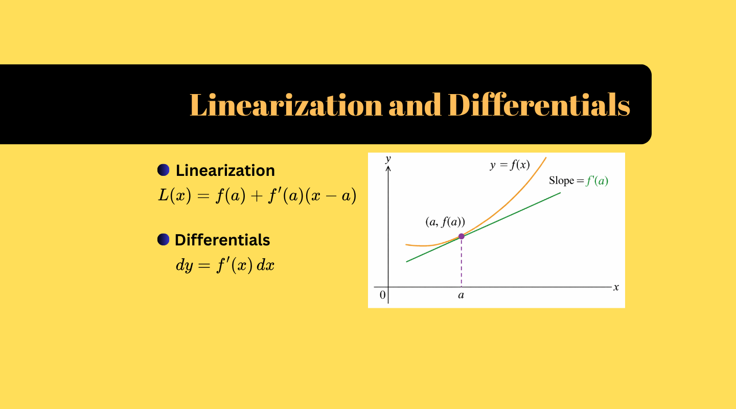
Suppose a function f(x) is differentiable at x=a. The derivative f'(a) represents the slope of the tangent line at that point. The equation of the tangent line at x=a is:
L(x) = f(a) + f'(a)(x - a)
This equation is called the linearization of f(x) at x=a. The function L(x) approximates f(x) when x is close to a. The closer x is to a, the more accurate the approximation becomes.
Why Linearization Works
The effectiveness of linearization comes from the definition of the derivative. The derivative measures the instantaneous rate of change of a function. Near the point x=a, the function changes almost at a constant rate equal to f'(a). Because of this nearly constant rate of change, the function behaves almost linearly over a small interval around a. This is why linear approximations are extremely accurate for small changes in x.
In AP Calculus, you are often expected to choose a value of a where the function is easy to evaluate, such as a perfect square, a multiple of \pi, or zero. This makes both f(a) and f'(a) simple to compute.
Geometric Interpretation of Linearization
Geometrically, linearization represents the tangent line to the curve at a point. On a graph, the curve and the tangent line intersect at the point (a,f(a)). Near this point, the tangent line lies very close to the curve. As you move farther away from a, the approximation becomes less accurate, and the tangent line begins to deviate from the curve.
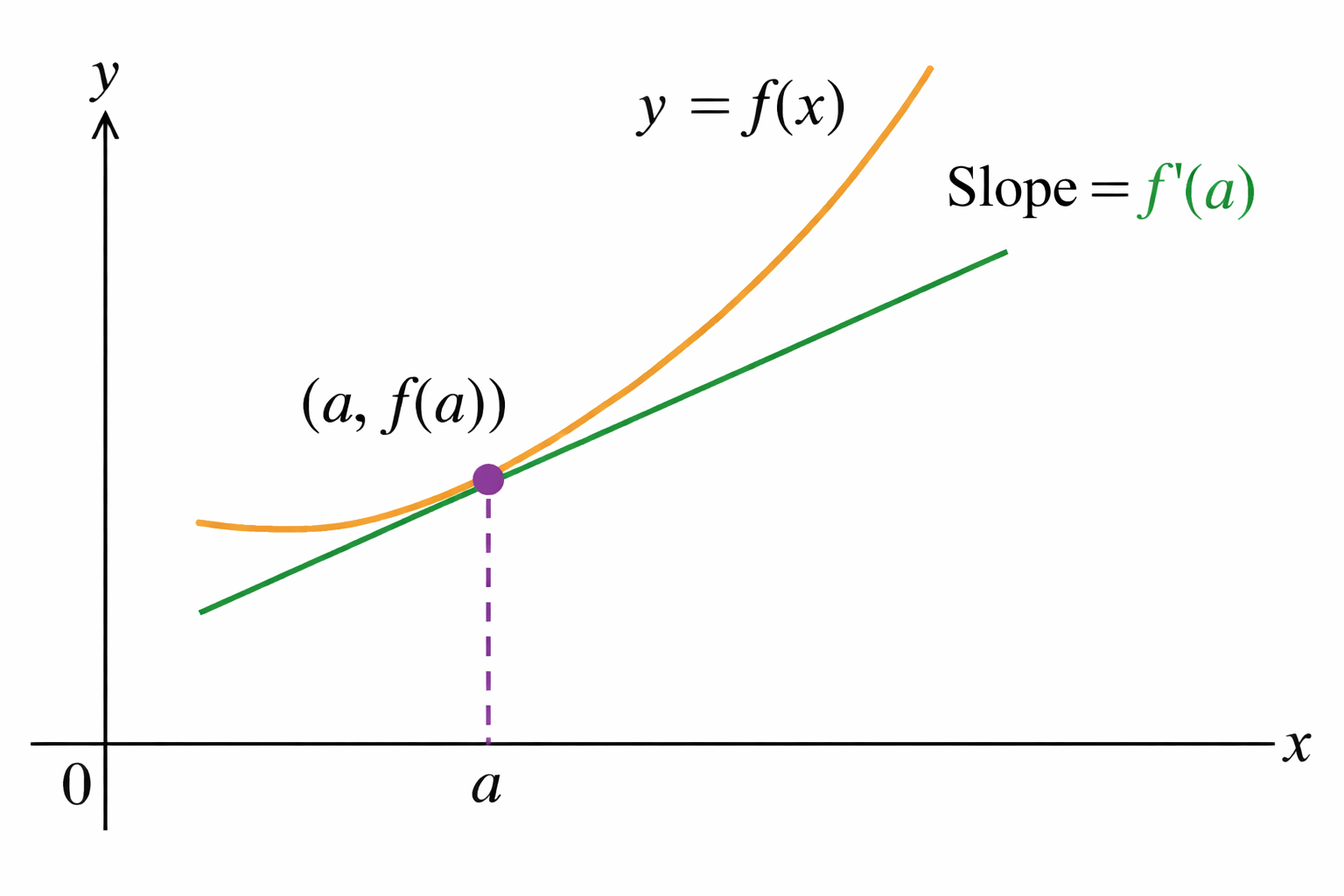
This geometric idea is crucial for understanding why linearization is a local approximation, not a global one. It works well only near the point of tangency.
Solved Example 1: Linearization
Approximate \sqrt{4.1} .
Step 1: Choose a nearby value
a = 4
Step 2: Define the function
f(x) = \sqrt{x}
Step 3: Find the derivative
f'(x) = \dfrac{1}{2\sqrt{x}}
Step 4: Evaluate at x=4
f(4) = 2, \quad f'(4) = \dfrac{1}{4}
Step 5: Linearization
L(x) = 2 + \dfrac{1}{4}(x - 4)
Approximation:
\sqrt{4.1} \approx 2.025
What are Differentials?
Differentials provide another way to understand linear approximations. Let y = f(x) .
If dx is a small change in x , then the differential of y is:
dy = f'(x)\,dx
Differentials give an approximate change in the output of a function based on a small change in the input. This concept is extremely useful in applications involving measurement errors and approximations.
Relationship Between Linearization and Differentials
Linearization and differentials are closely related. The expression:
f(x+dx) \approx f(x) + dy
shows that the change predicted by the tangent line is exactly the differential dy. In other words, differentials represent the change predicted by linearization.
Solved Example 2: Differentials
Estimate the change in y = x^2 when x changes from 3 to 3.02.
f'(x) = 2x
f'(3) = 6, \quad dx = 0.02
dy = 6(0.02) = 0.12
Estimated change in y: 0.12
Application: Error Estimation
One of the most important applications of differentials is error estimation. In real-life measurements, exact values are rarely known. If dx represents a small measurement error in x, then the approximate error in y is given by:
|dy| = |f'(x)|\,|dx|
This method is widely used in physics, engineering, and applied sciences and appears frequently in AP Calculus AB exam questions.
Solved Example 3: Error Estimation
A sphere has radius 5 cm with a possible error of 0.1 cm.
Estimate the maximum error in its volume.
V = \frac{4}{3}\pi r^3
dV = 4\pi r^2 dr
dV = 4\pi(5)^2(0.1) = 10\pi
Maximum error: \approx 31.4 \,\text{cm}^3
This method is widely used in physics, engineering, and applied sciences and appears frequently in AP Calculus AB exam questions.
Fully Solved Practice Questions
Question 1
Approximate \sqrt{15.9} using linearization at x=16.
Solution:
f(x)=\sqrt{x}, \quad f'(x)=\frac{1}{2\sqrt{x}}
L(x)=4+\frac{1}{8}(x-16)
\sqrt{15.9} \approx 3.9875
Question 2
A cube has side length 10 cm with error 0.2 cm. Estimate maximum error in volume.
Solution:
V=x^3 \Rightarrow dV=3x^2dx
dV=3(10)^2(0.2)=60
Question 3
Find linearization of f(x)=\sin x at x=0
Solution:
f(0)=0, \quad f'(x)=\cos x \Rightarrow f'(0)=1
L(x)=x
Question 4
Approximate (1.02)^5 using differentials.
Solution:
y=x^5, \quad dy=5(1)^4(0.02)=0.1
(1.02)^5 \approx 1.1
Frequently Asked Questions (FAQs)
Q1: What is linearization in calculus?
Linearization is a method used to approximate a complicated function by a linear function near a specific point. It uses the equation of the tangent line at that point to estimate nearby function values. Linearization works best when the input value is very close to the point of approximation.
Q2: Why does linearization give good approximations near a point?
Linearization works because a differentiable function behaves almost like a straight line when viewed very close to a point. Since the derivative represents the slope of the tangent line, the linear function closely matches the curve near that point.
Q3: What is the difference between linearization and differentials?
While differentials estimate the change in the function caused by a slight change in the input, linearization offers an approximate formula for the function itself. Actually, differentials show the change that the linearization predicts.
Q4: Is linearization included in AP Calculus AB exams?
Yes. Linearization and differentials are important topics in AP Calculus AB. Exam questions often test approximation, error estimation, interpretation of tangent lines, and conceptual understanding of derivatives.
Conclusion
Linearization and differentials allow us to simplify complex functions using tangent lines and derivatives.
These tools are essential for approximation, error estimation, and success in AP Calculus AB.